
Generation of high definition map for accurate and robust localization
 0
0Abstract
This paper presents a framework for generating high-definition (HD) map, and then achieves accurate and robust localization by virtue of the map. An iterative approximation based method is developed to generate a HD map in Lanelet2 format. A feature association method based on structural consistency and feature similarity is proposed to match the elements of the HD map and the actual detected elements. The feature association results from the HD map are used to correct lateral drift in the light detection and ranging odometry. Finally, some experimental results are presented to verify the reliability and accuracy of autonomous driving localization.
Keywords
1. INTRODUCTION
In recent years, vehicle localization has been treated as an important part of an autonomous driving system. However, conventional odometry methods have drift problems with long-term use. An inertial navigation system (INS) will likely fail in scenarios with poor GNSS signals, such as tunnel and urban canyon scenarios[1]. For the sake of more accurate localization, multisensor fusion is developed to compensate for the respective deficiencies of various sensors. HD maps, as stable prior information, can provide reliable location constraints. Fusion localization methods based on HD maps have been a significant research hotspot in recent years.
For HD maps, some computer-aided generation methods have emerged[2, 3]. However, lane lines obtained using these methods are a series of 2-dimensional point sets, which occupy large storage space and do not carry elevation information. Some researchers store road features in point clouds and use point cloud registration methods to determine vehicle positions[4, 5]. However, point cloud formats have disadvantages such as high coupling, difficulty in maintaining, and unfavorable object classification. For localization, some researchers reduce localization errors by matching road surface features, e.g. manhole covers[6–12]. However, the visibility of road features is easily affected by illumination, which makes the matching performance differ greatly at different times and results in unstable localization.
In this paper, the main work focuses on two aspects: First, a computer-aided generation method for HD maps is proposed. Currently, most papers consider the lane lines are in 2D plane when the lane line fitting is implemented. These methods are almost unusable in scenarios such as overpasses and culverts[13–16]. To broaden the use of HD maps, it is necessary to develop 3D fitting lane lines. Second, an accurate multisensor fusion localization method using generated HD map and existing odometry is proposed. It is worth noting that cumulative errors will occur if the localization method is only based on odometry. Thus, a positional constraint that has no connection with error is required to correct the estimated position. The contributions of this paper are summarized as follows:
1. We propose a method based on an iterative approximation to generate the 3D curve of lane lines. The spatial parameterized curve fitted by the proposed algorithm, which is global
2. We separate the lanes and store them in a particular HD map format instead of holding them as semantic information in a point cloud. For the HD maps nonuniform sampling point problem, a method based on numerical integration is proposed to achieve uniform sampling over the arc length.
3. We propose a method to associate the elements in the HD map and the other elements in the perception results.In this paper, the basic elements of the HD map and the complete feature associations are formulated with their respective similarity evaluation metrics, considering the matching time, similarity and local structure consistency.
4. We transform the localization problem of fusing HD maps into a graph optimization problem. Based on the HD map and perceptual image feature association results, a lateral constraint is applied to the odometry localization results, and accurate, low-cost localization results are obtained.
2. RELATED WORKS
2.1. Generation of lane curve equations
Chen et al.[14] demonstrated that a cubic Hermite spline (CHS) can describe line segments, arc curves, and clothoids simultaneously and is a good choice for fitting lane lines. A CHS has at least
2.2. Existing HD map formats
There is no unified standard for HD map formats, and various institutions and companies use different formats. The OpenDRIVE standard, developed by the Association for Standards in Automation and Measurement Systems (ASAM), has been used in simulations for some time and has good landing performance in some assisted driving models. The Navigation Data Standard (NDS) is a standard format for vehicle-level navigation databases jointly developed and published by vehicle manufacturers and automotive suppliers. The NDS format enables sharing of navigation data between different systems by separating the navigation data from the navigation software. Although OpenDRIVE and NDS are formats developed by more authoritative organizations, they need to be more open, as they provide only partial information to most developers. Therefore it is challenging to use them in practice[18, 19].
Apollo OpenDRIVE is a modified version of OpenDRIVE to accompany the Baidu Apollo autonomous driving system. Instead of using geometric elements, it uses sequences of points to represent road elements. In addition, Apollo OpenDRIVE stores reference lines on the map and then describes the lane lines relative to the reference lines. This allows Apollo OpenDRIVE to express maps with higher accuracy than OpenDRIVE for the same map file size and also facilitates some calculations in the subsequent planning module.
In 2018, Poggenhans et al.[20] released the open source Lanelet2. Based on the OpenStreetMap (OSM) format, Lanelet2 has been extended and allowed direct access to many of the open source tools that accompany OSM. Benefiting from its complete toolkit, open architecture, and easily editable features, Lanelet2 not only allows the storage of information about roads, road signs, light poles, and buildings with precise geometry but also enables lane level and traffic-compliant routing.
2.3. Multisensor fusion localization
GNSS are widely spread in intelligent transport systems and offer a low-cost, continuous and global solution for positioning[21]. It can provide a more stable location. GNSS localization system has obvious disadvantages: significant errors and easy to be obscured. Therefore, scholars have increasingly recognized multisensor fusion as necessary in recent years. Simultaneous localization and mapping (SLAM) is a technology that constantly builds and updates environmental information by sensing things in an unknown environment while tracking their position in the background. SLAM is generally divided into light detection and ranging (LiDAR)-based SLAM, such as LOAM[22], LeGO-LOAM[23], LINS[24], and LIO-SAM[25], and vision-based SLAM, such as ORB-SLAM[26], VINS[27, 28]. If the localization relies solely on LiDAR or cameras, position estimation errors will accumulate over a long time and distance. An HD map, as a globally consistent data source, can also provide reliable global location constraints. Multisensor fusion localization algorithms combined with HD map lane-level localization algorithms will be more accurate and have great potential.
2.4. Localization based on HD map
Scholars continue to reduce the error by matching pavement marking features or lane line curvature based on existing localization[6–12]. However, the visibility of road markings is affected by light. The visibility of different markings on the same road segment varies greatly at different periods, making it difficult to achieve stable positioning performance. At the same time, these efforts do not consider the common function of road elements in localization and planning, and these methods can only use the generated road elements in localization.
3. SYSTEM OVERVIEW
The proposed system consists of three parts. The first part is lane line fitting. An inverse lane line perspective mapping method combined with ground equations is discussed. An iterative approximation-based process of fitting piecewise CHS curves is proposed. This method satisfies the requirement of small data storage and ensures the continuity of lanes.
The second part is the HD map postprocessing. The data structure and coordinate system required for the HD map are discussed. We use a numerical integration method to calculate the parametric curve arc lengths. In this way, the parametric scale equidistant curves are transformed into arc-length scale middle curves, making the curve structure more uniform.
The third part is a fusion localization method based on HD maps and odometry. A method for feature association between current HD map information and the camera's real-time perceptual features is investigated. A respective similarity evaluation metric is formulated for different essential elements in the HD map. According to the accumulated confidence smoothing, the results are smoothed on the time scale and converted into a graph optimization problem. Finally, the amount of computation for graphics optimization is reduced using a sliding window method and improved keyframe selection.
The KITTI dataset is used for autonomous driving and mobile robot research[29]. This study uses only camera 2 and the synchronized and corrected data in the KITTI dataset. Therefore, we add some definitions based on KITTI's original definitions. Taking camera 2 as the origin to establish a camera coordinate system, the intersection of the vertical line from the midpoint of the front and rear axles of the vehicle (the middle of the four wheels) to the ground and the ground is taken as the vehicle center point, and the base_link coordinate system is established. The positive direction of the
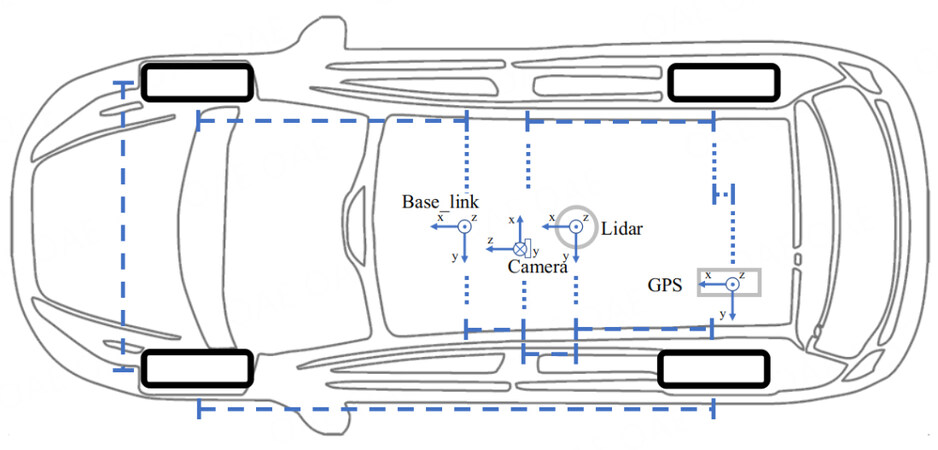
Figure 1. The coordinate system of the vehicle.
4. HD MAP GENERATION
We discuss the generation of HD maps with the lane line detection results already available from existing experimental data, and the test images are from the KITTI dataset[29]. An example of lane line data is shown in Figure 2. The lane line data are stored as line segments. Each segment is a lane consisting of several points.
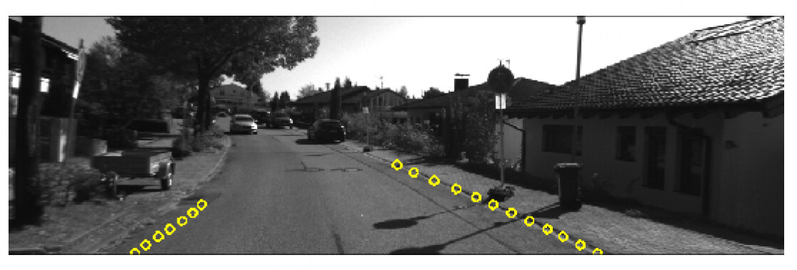
Figure 2. Lane detection data.
4.1. Inverse perspective mapping with ground equation
The projection equation of the camera is as follows:
where
We calculate the ground equations in the LiDAR coordinate system as follows[30]:
where
Combining (1) and (2),
where
The physical meaning of
Since the matrix
From (5), the program only needs to compute
4.2. Piecewise cubic hermite spline fitting
A CHS curve is a cubic polynomial curve determined by the starting point
(6) represents the equation of the
The problem of fitting the
It is evident that in each segment of the curve except the first one, only the endpoint tangent vector
An algorithm for fitting a piecewise spatial CHS curve is proposed based on the idea of asymptotic approximation, as shown in the Algorithm 1. The main idea of the algorithm is to cyclically optimize
Algorithm 1 CHS Curve Fitting with Asymptotic Approximation
for
for
if
end if
end for
end for
return
The traditional piecewise cubic Hermite interpolating polynomial (PCHIP)[32] algorithm fits a set of curves with four parameters every two points, so the number of parameters to be fitted increases exponentially with an increasing number of sampling points. The asymptotic approximation of the CHS curve fitting algorithm proposed in this section adds several sampling points to the curve fitting equation as constraint terms, which can effectively reduce the total number of parameters while ensuring that the curve is as close as possible to the remaining sampling points. As shown in Figure 3, the gray line is the actual curve, the red line is composed of 20 sampling points, and the blue and green lines are the curves fitted by the algorithm in this study. The smooth and continuous connection between the blue and green lines is evident in Figure 3. This shows that the algorithm's results in this study can still guarantee a certain accuracy in the case of more serious disturbances. This accuracy satisfies the need for lane line fitting.
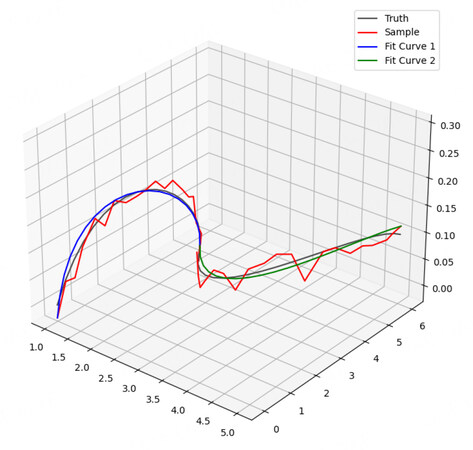
Figure 3. Curve fitting.
4.3. Intersection completions
Considering that some roads prohibit left or right turns, it is not feasible to fix intersections through geometric relationships. In this study, we evaluate the intersection connection using the trajectory information of the vehicle driving. The vehicle driving trajectory is superimposed on the set of lane points. When the lane points near the vehicle driving route are less than a threshold value, the intersection is considered to be at that point.
The parameters of a CHS curve equation in an intersection (called virtual lanes) can be determined by combining the endpoint of the departure lane and its tangent vector with the start point of the entry lane and its tangent vector. That is, for the equation of virtual lanes at this intersection, the equation of a lane line in intersection
4.4. Arc length equalization of curves
In Lanelet2, a sequence of points is used to describe lane lines. This storage method has some advantages; path-planning algorithms with some processing can use this point sequence. In addition to manual adjustment to edit HD maps, they must also manipulate the point sequence and cannot be operated on the parameterized curve. In contrast, some scenarios require global smoothing of curves, such as lane visualization drawing. Therefore, lane parameters and point sequences are stored in the map file in this study. Optimizing the curve equation after parameter
The CHS arc lengths can be calculated from the following equation:
(9) is an elliptic integral, which is difficult to calculate by ordinary methods. In this study, the Gauss-Kronrod quadrature method[33] is used to simplify the integration calculation process.
We use the G7-K15 method, a 7-point Gauss rule with a 15-point Kronrod rule, apply it to (9), and use the rules of the upper and lower limits of the integral transformation to calculate the arc length from
(10) can be used to calculate the arc length of the lane curve, which is not only used for equidistant sampling but also in intersection steering scenarios. The arc length can also be used to calculate curvature, which is convenient for planning.
5. LOCALIZATION BASED ON AN HD MAP
There are a variety of complex road environments in the cities, such as tunnels, overpasses, and urban canyons. These environments make GNSS-based localization less reliable. Some odometry fusing methods have emerged to solve the problem of GNSS failure. However, due to odometry drift, these methods cannot meet the localization requirements in scenarios where there is a long-term lack of effective global position information[34]. Although point cloud map relocalization based on the iterative closest point (ICP)[35], normal distribution transform (NDT)[36] and other methods is very effective, a very large point cloud map becomes a major challenge that affects practical use. An HD map contains various semantic features, while lane lines and traffic signs have good recognition both day and night. To explore the global localization method combining an HD map and IMU, two problems need to be solved. First, the elements in the HD map are associated with the elements detected using other sensors. Second, the pose is estimated based on the feature association results.
5.1. Reprojection
Reprojection refers to projecting the coordinates of a corresponding point in 3D space back to the pixel plane according to the currently estimated pose. The error between the reprojected and actual pixel coordinates is called the reprojection error and is often used as an indicator to evaluate the pose. Based on the position of the lane in the map, the known a priori knowledge of the HD map is projected onto the camera image by combining the intrinsic and extrinsic parameters of the camera. The evaluation of a pose metric is obtained by differencing the a priori map element positions and the coordinates of the matching perceptual results. Ideally, the distance between the two should be zero. The optimal camera pose can be obtained by optimizing the camera pose using a nonlinear optimization method to minimize this evaluation metric so that the optimal vehicle pose can be calculated.
First, referring to the transcendental vehicle pose
where
5.2. Feature association
To use an HD map for localization, the location of objects detected by the sensors on the HD map needs to be known. This step is called feature association. Feature association locates HD map elements that match the features detected in the camera images. The correct selection of map features can significantly improve the localization results. In this study, we choose lane line elements as map features. This is because lane line features are easy to detect, have a long duration, and have good reflection properties, and have a high detection success rate in environments such as nighttime. The map elements are reprojected to the pixel plane (map features), and the distance between the detected elements (perceptual features) is calculated and used to evaluate the localization results.
Define the perceptual feature
Based on the consistency of the local structure, the map feature reprojection error is calculated. Then, coarse matching of features and HD map perceptual features is performed. If the reprojection error is too large, the gap between the map and perceptual features is considered too large and will not be matched and optimized. The algorithm continues only when the error is less than a certain threshold. Define the map feature as
For the lane lines, define the likelihood probability
where
Considering the map structure consistency, the perceptual feature structure should be similar to the map feature structure. After coarse matching, the distance between two of each map feature and the distance between two of the matching perceptual features is calculated, as shown in Figure 4. These two sets of distances are called the structural features of the map features and the structural features of the perceptual features. The difference in the structural features is used as a measure to assess the similarity between a given frame's perceptual feature structure and the map feature structure.
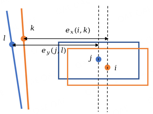
Figure 4. Edge similarity definition
Define the matching matrix
where
Considering the number of matches, structural consistency, and reprojection error, the feature matching problem can be expressed as a multi-order map matching problem.
where
5.3. Factor graph optimization
Define known sensor measurements
This MAP estimation can be decomposed into two subproblems, feature association and pose estimation, to create a feature association
We use factor graphs to optimally fuse odometry
The above equation splits the MAP estimation into the product of the maximum likelihood estimate (MLE) and the prior. Therefore, (17) can be equated to an MLE problem. Therefore, the pose
Assume that the noise satisfies a normal distribution. The odometry error optimization term can be defined as:
where
The landmark error optimization term can be defined as:
where the landmark error can be represented by the difference between the
The map error optimization term can be described as[37]:
where
When the error of a particular edge is significant, the growth rate of the Mahalanobis distance in the above equation is substantial. Therefore, the algorithm will try to preferentially adjust the estimates associated with this edge and ignore the effect of other advantages. This study uses the Huber kernel function
Combining (19), (21), and (23), the pose optimization function is obtained as follows:
6. EXPERIMENTS AND RESULTS
We validated the proposed localization algorithm through a series of experiments. First, the KITTI dataset is gradually simplified to fit a single parametric curve based on various lane characteristics. The curve equation of each lane line is calculated based on the three-time Hermite spline curve fitting algorithm proposed in this paper. Then, after intersection complementation and manual adjustment of elements, an HD map corresponding to the KITTI dataset is generated. Finally, based on the original odometry, the priori HD map information and the fused HD map localization algorithm proposed are used to further constrain the vehicle's lateral position.
6.1. Curve fitting
To fit the lane lines, we must extract the lane points. The first step uses the ground plane fitting (GPF) algorithm[30] to calculate the ground equation. The coordinates of the lane lines on the image in the camera coordinate system
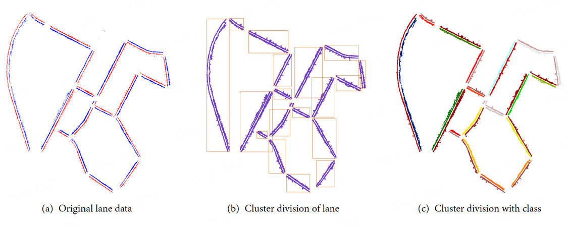
Figure 5. Extract lane points.
The second step uses density-based spatial clustering of applications with noise (DBSCAN)[39] clustering to divide the closely spaced points (distance less than a certain threshold) into the same cluster. This search threshold needs to be slightly greater than the lane spacing and less than the distance between adjacent lanes at an intersection. This enables the clustering algorithm to search for adjacent lanes and ensure that the intersection area can be used for segmentation. Because of the large number of point clouds, the KD-Tree search algorithm is used rather than a traditional traversal search. Through DBSCAN clustering, the lane lines are divided into 19 areas, as shown in Figure 5(b).
In the third step, the lanes are divided via DBSCAN clustering using the information of different lanes in the same road recorded in the first step. Then the lanes are divided according to the category attribute for each segment, as shown in Figure 5(c). A unique ID is assigned to each lane here for subsequent lane completion.
The curve fitting process is shown in Figure 6, where the upper left, middle and right are X-Y, X-Z, and Y-Z views, respectively, which show that the fitting effect is relatively good. The spatial curve can describe the original lane line point set better.
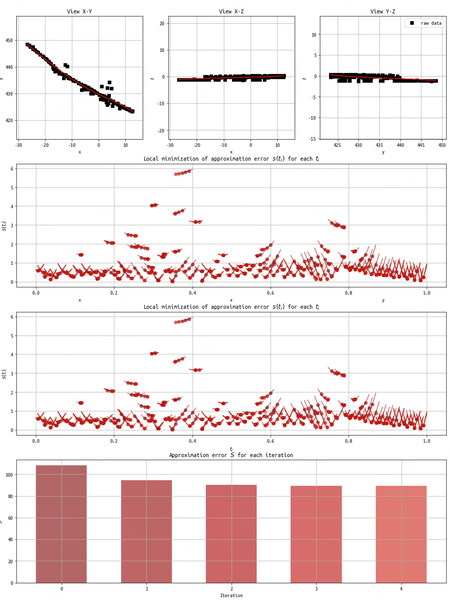
Figure 6. Curve fitting process.
The middle subplot of Figure 6 shows the fitting effect of parameter
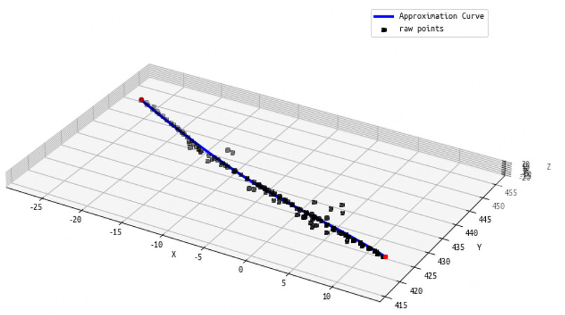
Figure 7. Single lane fitting result.
This study determines the intersection connection based on the vehicle path to solve the problem that there may be no left turn or right turn on the road. The intersection topology is selected by combining the IDs assigned to each lane. The algorithm completes the virtual lane lines of the intersection.
The results before and after intersection completion are shown in Figure 8(a). The final lanes for the entire area are shown in Figure 8(b), and the overall lane fit is relatively good. To create an HD map, further manual adjustment of the lane curve is also required, and complements other elements on the map, such as sidewalks and various traffic signs.
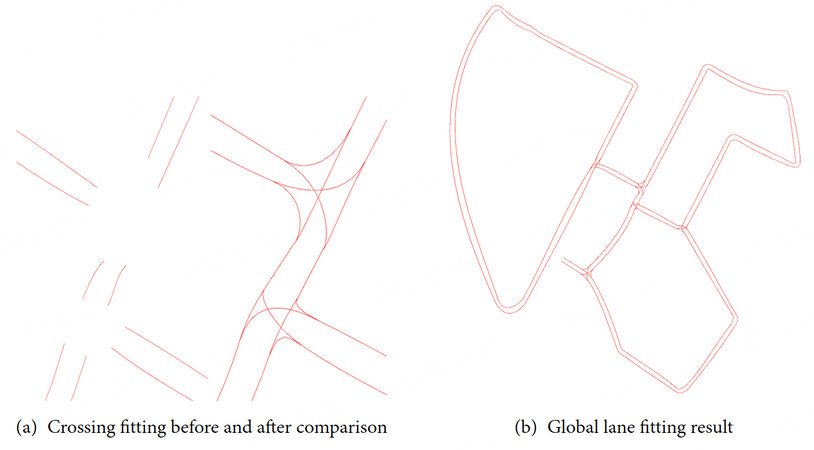
Figure 8. Lane Fitting Process
6.2. HD map production
The vehicle's starting point is defined as the map origin, and the GPS coordinates of the origin (48.982 545 °W, 8.390 366 °E) are recorded. To obtain higher projection accuracy, the European ETRS89 coordinates are used in this study. The coordinate system parameters are shown in Table 1.
ETRS89 coordinate System
| Name | Value |
| EPSG number | EPSG: 25832 |
| Prime meridian | Greenwich |
| Earth's ellipsoid | GRS 1980 (long axis: 6, 378, 137 m, flat rate: 298.257, 222) |
We import the long-axis flattening of the Earth ellipsoid defined by the ETRS coordinate system in Table 1 into the Geographiclib geographic coordinate library for calculation. The coordinates of the initial point in the MGRS geographic coordinate system are 32UMV-55394.36-25694.44, of which the area number is 32UMV, the distance to the east is 55394.36 m, the distance to the north is 25 694.44 m, and the grid north angle is
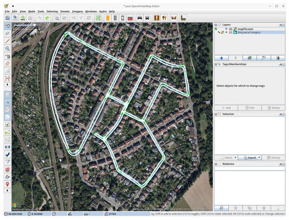
Figure 9. The lanelet2 map.
Figure 8(b) shows that some intersections are poorly fitted. The elements, such as stop lines and crosswalks, are not identified. Therefore, some elements that were missed by mistake were manually adjusted, the lane shape was fine-tuned, and pedestrian crossing markings and some traffic signs were added. Figure 10 shows the effect of manual labeling of some intersections. After adjusting the lane lines, a new curve equation needs to be refitted for this lane using the method in Part IV. Finally, the lane curve is optimized using a numerical integration method to approximate the arc-length isometric sampling.
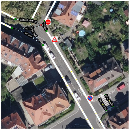
Figure 10. Manual marking.
6.3. Localization experiment
Following the previous preparations, the next step is to conduct a localization experiment. The points of the HD map are projected in the image coordinate system using formula (11). Considering the actual lanes in the camera image orientation, only the lanes located in the lower half of the image are kept, as shown in Figure 11. Since the virtual lane (blue) in the figure should not be involved in matching and optimizing the position attitude, only the actual lane (red) is reserved for lane matching and position optimization. The horizontal red lanes on both sides result from the projection of the nearby road, not the current road. The algorithm filters the possible lanes by radius and then projects them into the image. The final lanes involved in matching are shown in Figure 12.
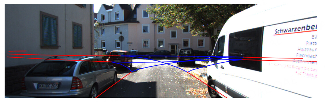
Figure 11. The reprojection of HD map.
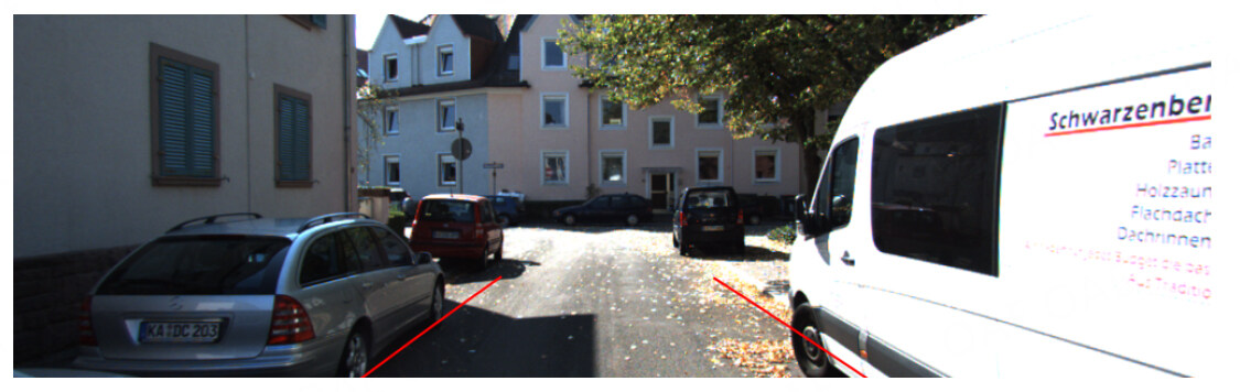
Figure 12. Available lanes for matching and optimizationp.
Because the inertial guidance odometry in the KITTI dataset is relatively accurate, it does not reflect the effect of the localization algorithm well. In this paper, we use the LOAM[22] algorithm as a laser odometry and match the HD map with the actual detection results using the method proposed in Part V. The obtained matching results are added to the Georgia Tech Smoothing and Mapping (GTSAM)[40] optimization as roadmap constraints. To test the effect of fused localization, the fused HD map localization algorithm designed in this study is compared with the comparison of the actual value, as shown in Figure 13.
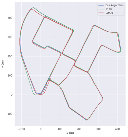
Figure 13. Comparison between our algorithm, LOAM and the ground truth.
The metric commonly used in academia to evaluate trajectories is the root-mean-square deviation (RMSE):
The absolute pose error (APE) considers only translational errors:
In this study, the EVO[41] toolkit is used to evaluate the trajectory error of the proposed localization algorithm, and the results are shown in Table 2.
Localization error
| Algorithm | RMSE | Min APE error | Max APE error |
| Algorithm of this paper | 4.3361m | 0.6679m | 15.1492m |
| LOAM | 12.5518m | 1.1545m | 21.8804m |
Figure 13 shows the comparison of the effect of the proposed algorithm and the LOAM algorithm. The proposed localization algorithm has a more significant improvement compared to the pure LOAM distance meter. As seen, the error in the localization effect of incorporating the HD map remains small most of the time. A horizontal offset can be seen in the upper left part of the road where the HD map does not exist. Because the leftmost road is long and has a particular curvature, the localization of the fused HD map needs to be improved for the forward direction. The LiDAR odometer has a large offset on the lower left side of the road, so the algorithm developed in this study also has a large offset. This problem can be solved by subsequently considering adding more road elements.
6.4. Robustness test
Now, we compare the localization performance of the method in this paper with other methods. Since the road in the experimental scenes is lined with trees, the features extracted by LiDAR from the dense foliage are very noisy. In the experimental scenes, the GPS localization is correct because the GPS signal completely covers the experimental data set. We treat the GPS measurements here as ground truth. Figure 14(b) shows the localization results of the method in this paper with other methods in this case. LIOM lacks a pre-processing method to filter out reliable features, so its results are far from the correct ones. The unsatisfactory LIO-SAM results are due to unreliable features that severely affect the matching between keyframes. The method in this paper can obtain more accurate results than other methods.
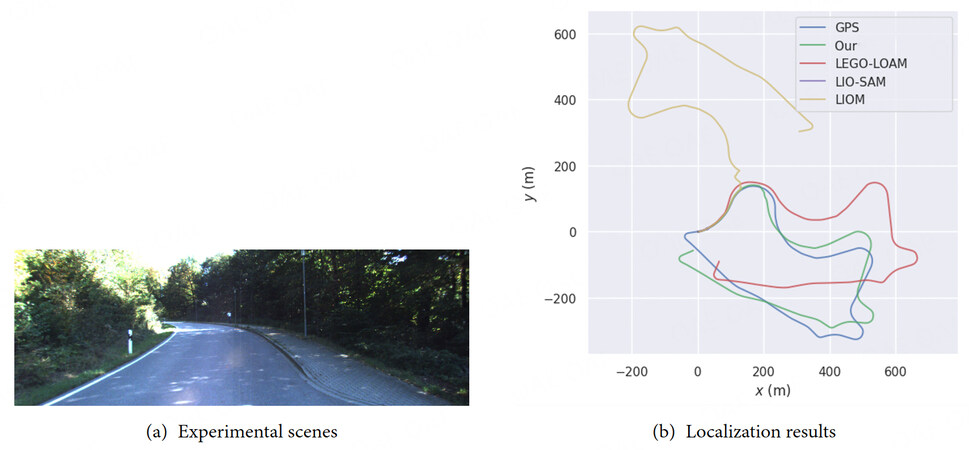
Figure 14. Robustness test.
7. CONCLUSION
In this paper, an iterative approximation-based method is proposed to generate the 3D curves of lane lines. For the problem of uneven sampling points in HD maps, a method based on numerical integration is proposed to achieve uniform sampling over the arc length. Based on the feature association results of the HD map and the perceptual image, lateral constraints are applied to the odometer localization results to obtain accurate and low-cost localization results. Experimental results show that the proposed method can generate HD maps and achieve high-precision localization. Future work will try to consider the lateral serial numbers of lane lines for clustering. Larger thresholds are easier to cluster on lane points with the same serial number. The radius threshold of lane points with different serial numbers is reduced so that the clustering can be clustered along the direction of lane lines, which can solve the problem of intermittent lane lines. To improve the practicality of this method, we will continue to explore the detection of more road elements, the generation of topological relationships for complex road sections (e.g., traffic circles), and the automatic association methods of traffic signs and lanes in the future. The main sensors used in this system are LiDAR and camera, which are sensitive to rain and snow occlusion. Therefore, the present system is not robust in rain and snow environment. In the subsequent work, thanks to the graphical optimization framework, we can easily add GPS measurement constraints to the position map. This can overcome the effect of rain and snow environment on the system to some extent. Cloudy weather is still one of the important challenges for GPS localization systems. In future work, we will add kinematic model constraints to improve GPS localization results.
DECLARATIONS
Authors' contributions
Writing-Original Draft and conceptualization: Huang Z
Technical Support: Chen S
Validation and supervision: Xi X, Li Y
Investigation: Li Y, Wu S
Availability of data and materials
Not applicable.
Financial support and sponsorship
This work was supported by the Open fund of State Key Laboratory of Acoustics under Grant SKLA202215.
Conflicts of interest
All authors declared that there are no conflicts of interest
Ethical approval and consent to participate
Not applicable
Consent for publication
Not applicable
Copyright
© The Author(s) 2023.
REFERENCES
1. Jeong J, Cho Y, Shin YS, Roh H, Kim A. Complex urban dataset with multi-level sensors from highly diverse urban environments. Int J Robot Res 2019;38:642-57.
2. Azimi SM, Fischer P, Körner M, Reinartz P. Aerial LaneNet: lane-marking semantic segmentation in aerial imagery using wavelet-enhanced cost-sensitive symmetric fully convolutional neural networks. IEEE Trans Geosci Remote Sensing 2019;57:2920-38.
3. Fischer P, Azimi SM, Roschlaub R, Krauß T. Towards HD maps from aerial imagery: robust lane marking segmentation using country-scale imagery. IJGI 2018;7:458.
4. Cheng W, Yang S, Zhou M, et al. Road Mapping and Localization Using Sparse Semantic Visual Features. IEEE Robot Autom Lett 2021;6:8118-25.
5. Qin T, Zheng Y, Chen T, Chen Y, Su Q. RoadMap: A light-weight semantic map for visual localization towards autonomous driving. arXiv: 210602527[cs] 2021 Jun. Available from: http://arxiv.org/abs/2106.02527. [Last accessed on 29 Jan 2023].
6. Hosseinyalamdary S, Peter M. LANE LEVEL LOCALIZATION; USING IMAGES AND HD MAPS TO MITIGATE THE LATERAL ERROR. Int Arch Photogramm Remote Sens Spatial Inf Sci 2017;XLII-1/W1:129-34.
7. Matthaei R, Bagschik G, Maurer M. Map-relative localization in lane-level maps for ADAS and autonomous driving. In: 2014 IEEE Intelligent Vehicles Symposium Proceedings. MI, USA: IEEE; 2014. pp. 49–55. Available from: http://ieeexplore.ieee.org/document/6856428/. [Last accessed on 29 Jan 2023].
8. Nedevschi S, Popescu V, Danescu R, Marita T, Oniga F. Accurate Ego-Vehicle Global Localization at Intersections Through Alignment of Visual Data With Digital Map. IEEE Trans Intell Transport Syst 2013;14:673-87.
9. Qu X, Soheilian B, Paparoditis N. Vehicle localization using mono-camera and geo-referenced traffic signs. In: 2015 IEEE Intelligent Vehicles Symposium (IV); 2015. pp. 605–10.
10. Tao Z, Bonnifait P, Frémont V, Ibañez-Guzman J. Mapping and localization using GPS, lane markings and proprioceptive sensors. In: 2013 IEEE/RSJ International Conference on Intelligent Robots and Systems; 2013. pp. 406–12.
11. Welzel A, Reisdorf P, Wanielik G. Improving urban vehicle localization with traffic sign recognition. In: 2015 IEEE 18th International Conference on Intelligent Transportation Systems; 2015. p. 5.
12. Xiao Z, Yang D, Wen T, Jiang K, Yan R. Monocular Localization with Vector HD Map (MLVHM): A Low-Cost Method for Commercial IVs. Sensors (Basel) 2020;20:1870.
13. Jo K, Lee M, Kim C, Sunwoo M. Construction process of a three-dimensional roadway geometry map for autonomous driving. Proceedings of the Institution of Mechanical Engineers, Part D: Journal of Automobile Engineering 2017;231:1414-34.
14. Chen A, Ramanandan A, Farrell JA. High-precision lane-Level road map building for vehicle navigation. In: IEEE/ION Position, Location and Navigation Symposium; 2010. pp. 1035–42.
15. Jo K, Sunwoo M. Generation of a precise roadway map for autonomous cars. IEEE Trans Intell Transport Syst 2014;15:925-37.
16. Zhang T, Arrigoni S, Garozzo M, Yang Dg, Cheli F. A lane-level road network model with global continuity. Transportation Research Part C: Emerging Technologies 2016;71:32-50.
17. Gwon GP, Hur WS, Kim SW, Seo SW. Generation of a precise and efficient lane-level road map for intelligent vehicle systems. IEEE Trans Veh Technol 2017;66:4517-33.
18. Godoy J, Artuñedo A, Villagra J. Self-Generated OSM-Based Driving Corridors. IEEE Access 2019;7:20113-25.
19. Jiang K, Yang D, Liu C, Zhang T, Xiao Z. A flexible multi-layer map model designed for lane-level route planning in autonomous vehicles. Engineering 2019;5:305-18.
20. Poggenhans F, Pauls JH, Janosovits J, et al. Lanelet2: a high-definition map framework for the future of automated driving. In: 2018 21st International Conference on Intelligent Transportation Systems (ITSC). Maui, HI: IEEE; 2018. pp. 1672–79. Available from: https://ieeexplore.ieee.org/document/8569929/. [Last accessed on 29 Jan 2023].
21. Marais J, Ambellouis S, Flancquart A, et al. Accurate localisation based on GNSS and propagation knowledge for safe applications in guided transport. Procedia - Social and Behavioral Sciences 2012;48:796-805.
22. Zhang J, Singh S. LOAM: Lidar odometry and mapping in real-time. In: Robotics: Science and Systems. vol. 2. Berkeley, CA; 2014. pp. 1–9.
23. Shan T, Englot B. Lego-loam: Lightweight and ground-optimized lidar odometry and mapping on variable terrain. In: 2018 IEEE/RSJ International Conference on Intelligent Robots and Systems (IROS). IEEE; 2018. pp. 4758–65.
24. Qin C, Ye H, Pranata CE, et al. LINS: a lidar-inertial state estimator for robust and efficient navigation. In: 2020 IEEE International Conference on Robotics and Automation (ICRA). IEEE; 2020. pp. 8899–906.
25. Shan T, Englot B, Meyers D, et al. Lio-sam: Tightly-coupled lidar inertial odometry via smoothing and mapping. In: 2020 IEEE/RSJ International Conference on Intelligent Robots and Systems (IROS). IEEE; 2020. pp. 5135–42.
26. Campos C, Elvira R, Rodríguez JJG, M Montiel JM, D Tardós J. ORB-SLAM3: an accurate open-source library for visual, visual–inertial, and multimap SLAM. IEEE Trans Robot 2021;37:1874-90.
27. Qin T, Li P, Shen S. Vins-mono: A robust and versatile monocular visual-inertial state estimator. IEEE Trans Robot 2018;34:1004-20.
28. Qin T, Shen S. Online temporal calibration for monocular visual-inertial systems. In: 2018 IEEE/RSJ International Conference on Intelligent Robots and Systems (IROS). IEEE; 2018. pp. 3662–69.
29. Geiger A, Lenz P, Stiller C, Urtasun R. Vision meets robotics: the KITTI dataset. Int J Robot Res 2013;32:1231-37.
30. Zermas D, Izzat I, Papanikolopoulos N. Fast segmentation of 3D point clouds: a paradigm on LiDAR data for autonomous vehicle applications. In: 2017 IEEE International Conference on Robotics and Automation (ICRA). Singapore, Singapore: IEEE; 2017. pp. 5067–73. Available from: http://ieeexplore.ieee.org/document/7989591/. [Last accessed on 29 Jan 2023].
31. Byrd RH, Lu P, Nocedal J, Zhu C. A limited memory algorithm for bound constrained optimization. SIAM J Sci Comput 1995;16:1190-208.
32. Fritsch FN, Carlson RE. Monotone piecewise cubic interpolation. SIAM J Numer Anal 1980;17:238-46.
34. Wang H, Xue C, Zhou Y, Wen F, Zhang H. Visual semantic localization based on HD map for autonomous vehicles in urban scenarios. In: 2021 IEEE International Conference on Robotics and Automation (ICRA). Xi'an, China: IEEE; 2021. pp. 11255–61. Available from: https://ieeexplore.ieee.org/document/9561459/. [Last accessed on 29 Jan 2023].
35. Besl PJ, McKay ND. Method for registration of 3-D shapes. In: Sensor fusion IV: control paradigms and data structures. vol. 1611. Spie; 1992. pp. 586–606.
36. Biber P, Straßer W. The normal distributions transform: a new approach to laser scan matching. In: Proceedings 2003 IEEE/RSJ International Conference on Intelligent Robots and Systems (IROS 2003)(Cat. No. 03CH37453). vol. 3. IEEE; 2003. pp. 2743–48.
37. Wilbers D, Merfels C, Stachniss C. Localization with sliding window factor graphs on third-Party maps for automated driving. In: 2019 International Conference on Robotics and Automation (ICRA). Montreal, QC, Canada: IEEE; 2019. pp. 5951–57. Available from: https://ieeexplore.ieee.org/document/8793971/. [Last accessed on 29 Jan 2023].
38. Rusu RB, Marton ZC, Blodow N, Dolha M, Beetz M. Towards 3D Point cloud based object maps for household environments. Robot Auton Syst 2008;56:927-41.
39. Ester M, Kriegel HP, Sander J, Xu X. A density-Based algorithm for discovering clusters in large spatial databases with noise. In: Proceedings of the Second International Conference on Knowledge Discovery and Data Mining. KDD'96. AAAI Press; 1996. pp. 226–31.
40. Dellaert F. Factor graphs and GTSAM: a hands-on introduction. Georgia Institute of Technology 2012; doi: 10.1561/9781680833270.
41. Grupp M. Evo: Python package for the evaluation of odometry and SLAM.; 2017. Available from: https://github.com/MichaelGrupp/evo. [Last accessed on 29 Jan 2023].
Cite This Article
Export citation file: BibTeX | RIS
OAE Style
Huang Z, Chen S, Xi X, Li Y, Li Y, Wu S. Generation of high definition map for accurate and robust localization. Complex Eng Syst 2023;3:2. http://dx.doi.org/10.20517/ces.2022.43
AMA Style
Huang Z, Chen S, Xi X, Li Y, Li Y, Wu S. Generation of high definition map for accurate and robust localization. Complex Engineering Systems. 2023; 3(1): 2. http://dx.doi.org/10.20517/ces.2022.43
Chicago/Turabian Style
Huang, Zhengjie, Sijie Chen, Xing Xi, Yanzhou Li, Ya Li, Shuanglin Wu. 2023. "Generation of high definition map for accurate and robust localization" Complex Engineering Systems. 3, no.1: 2. http://dx.doi.org/10.20517/ces.2022.43
ACS Style
Huang, Z.; Chen S.; Xi X.; Li Y.; Li Y.; Wu S. Generation of high definition map for accurate and robust localization. Complex. Eng. Syst. 2023, 3, 2. http://dx.doi.org/10.20517/ces.2022.43
About This Article
Copyright

Data & Comments
Data
0

 Cite This Article 28 clicks

 Like This Article 19
likes
Like This Article 19
likes


Comments
Comments must be written in English. Spam, offensive content, impersonation, and private information will not be permitted. If any comment is reported and identified as inappropriate content by OAE staff, the comment will be removed without notice. If you have any queries or need any help, please contact us at support@oaepublish.com.